8 Google Sheets Hacks You’ll Wish You Knew Earlier

Not many people think of Google Sheets as an exciting app, let alone one that can help you save time. But there are many features, shortcuts, and surprising ways to use it that can help you be more productive — and even have some fun while you’re doing it.

Whether you’ve been using the app for years or are a complete beginner, these Google Sheets hacks will help you become a spreadsheet pro in no time. You’ll learn everything from basic shortcuts like randomizing names for contests to more advanced tips like applying conditional formatting and exporting metadata from websites in bulk.

Let’s get started!

1. Automate online research with PixieBrix

Maybe you're putting together a list of inspiring websites or a folder of affordable restaurants. Instead of switching back and forth between tabs, use PixieBrix's Quick Bar page to Google Sheets mod to send web page URLs and other page context directly to Google Sheets.

Here’s how to do it:

Download PixieBrix's Chrome extension
Make sure your Google Sheet has two columns: one named "Provider" and one called "URL"
Then, when browsing any webpage, simply right-click and type send page to Google Sheets
PixieBrix will automatically input the URL and provider name into your spreadsheet

You can also do even more in-depth research using Google Sheets and PixieBrix.

For example, you can populate Google Sheets with YouTube videos or multiple webpages' metadata (if you're doing SEO research). Or you can speed up vacation planning by bulk scraping data from Airbnb into a Google Sheet.

(Thanks, Google Sheets, for helping me find a tiny home rental in Idaho that is also built to look like a potato!) Learn more about our Google Sheets Integration here.

2. Drag cell data to continue patterns

Many Google Sheets users will already know this trick, but it’s so useful we think it’s worth a reminder.

Google sheets can recognize patterns pretty quickly. Next time you have to input some predictable data (e.g., days of the week or ascending numbers), note the blue square in the bottom right corner of your highlighted cell. Click on this and drag it down to new rows to apply the same values to them.

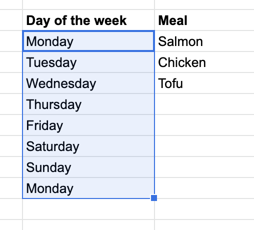
Dragging a column of cell data labeled "Day of the week" in Google Sheets, showing days of the week automatically populating

Doing this doesn't just copy the data into the new cells. It also predicts future data entries based on the ones you've highlighted, filling in any pattern you've established.

You can also do this with formulas. Apply the formula to your first cell and then drag it down to respond to each cell of data.

This Google Sheets hack will save you tons of time you might otherwise spend on manual data entry.

3. Randomize names and numbers

Randomizing names and numbers can be a helpful trick in a number of scenarios. Running a social media contest and need to pick a winner? Organizing your office’s Secret Santa and need to assign random pairs? (For the last time, you can’t buy the whole team shirts that say “Diehard is a Christmas movie,” Brenda!).

Google Sheets is here to help with a simple formula.

Here's how to pick a random name or number from a list in Google Sheets:

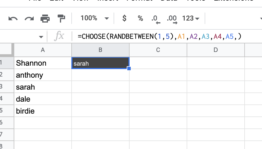
List your names or numbers in a column.
In a cell in the next column, paste this function snippet: =CHOOSE(RANDBETWEEN(1,4),A1,A2,A3,A4,)
Adjust the range (1,4) to the number of names in your sheet.
Click "Enter." A random name or number will appear in the column next to your list.

A Google Sheet showing 2 columns, one with a list of 5 names and one with one name chosen by the "Randomize" formula

4. Create a drop-down list

Maybe you’re creating a form for customers to submit, or you need team members to choose from a list of options for a project. Using a drop-down list will make it easy for people to select an answer without having to type it in.

This trick is most appropriate to use when you want to limit the options people can choose from and keep your spreadsheet from getting too chaotic.

Bonus: It's also helpful for impressing your colleagues with general spreadsheet wizardry.

To create a drop-down list in Google Sheets:

Select the cells where you want the list to appear (usually in a column)
Go to the “Data” tab and select “Data Validation”
By "Criteria," click "List of items"
List the items you would like to include in your drop-down list separated by commas
Click "Save"

And voila!

Your drop-down list should appear in the cells you've highlighted. Anything inputted in those cells that don't match the items you listed in "Criteria" will show up as invalid with a little red triangle in the top right corner of the cell.

5. View the edit history of a cell

Anyone who has collaborated on a Google Sheet with more than one person knows things can get a little chaotic, especially if everyone has editing permissions.

That’s why it’s helpful to be able to view the edit history of not just your whole document, but also individual cells. It’s especially helpful when working with formulas. Suddenly, it’s much easier to see where a mistake was made, as well as who made it, so everyone can learn from it.

Here’s how to do it:

Right-click on a cell
Select “Show edit history”
Click on the top right arrow to review past edits chronologically

6. Create trend heatmaps out of your data

Use conditional formatting to change the color of cells based on their value, or to create rules for automatically highlighting cells that meet certain conditions. This is helpful for quickly understanding large data sets and for spotting patterns that would be otherwise difficult to see.

For example, if you’re comparing sales for a set of products year-over-year, you could use conditional formatting to automatically color products that have increased in sales green and products that have decreased in sales red.

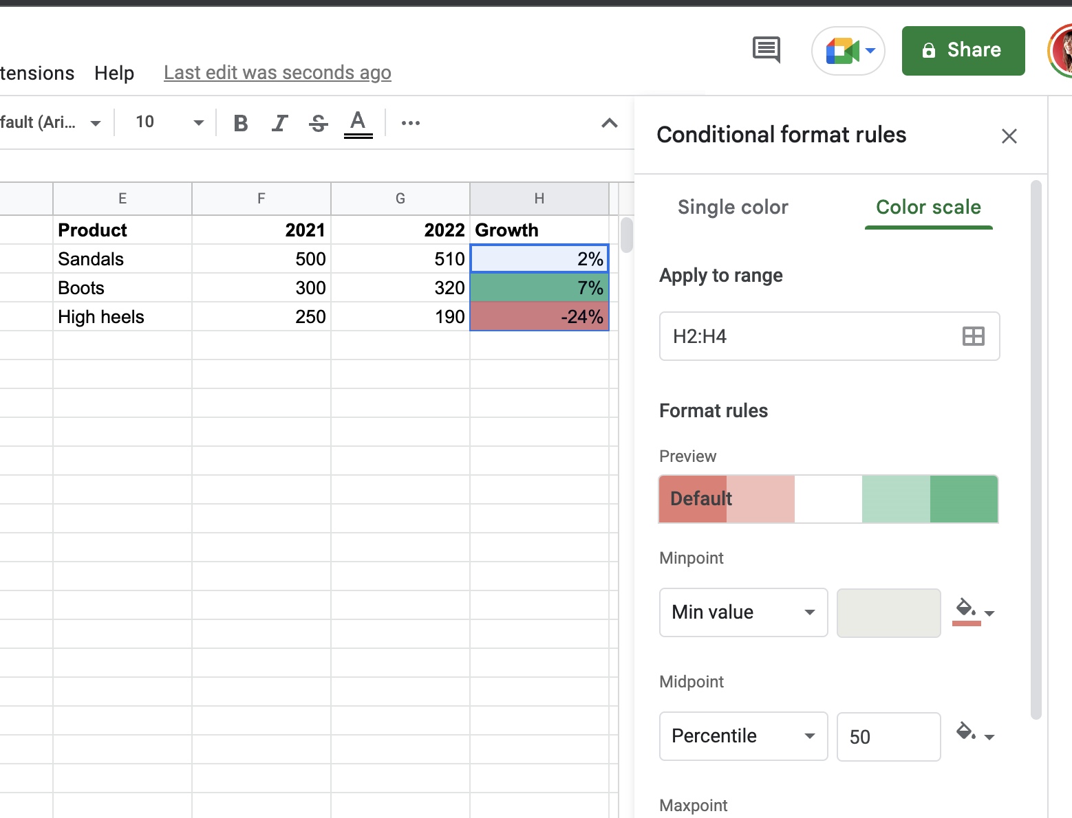
A Google Sheet showing a column of numbers to which conditional formatting has been applied. Numbers above zero are formatted in increasingly dark green, while the negative number is formatted red.

To use conditional formatting to highlight trends this way:

Select the cells you wish to format
Go to “Format,” the “Conditional Formatting”
Choose “Color scale”
Under “Format rules,” select the color spectrum you want
Ensure the Midpoint value is set to “Percentile” and at 50 (or whatever the midpoint number of your list is)

7. Use common keyboard shortcuts

Real Google Sheets pros know their keyboard shortcuts. That’s because it’s one of the laziest/easiest ways to save time.

Just dipping your toes into keyboard shortcuts? Here is Google’s official list for Mac and Windows users.

Here are some of our time-saving favorites for Windows:

Insert rows above the current row: Ctrl-Alt-Shift-Equals sign
Insert rows below the current row: Alt-i-W (Google Chrome) or Alt-Shift-i-W
Insert columns to the left of the current column: Ctrl-Alt-Shift-Equals sign
Insert columns to the right of the current column: Alt-i-O (Google Chrome) or Alt-Shift-i-O
Delete rows or columns: Ctrl-Alt-Minus

And for Mac:

Insert rows above the current row: Command-Option-Equals sign
Insert rows below the current row: Ctrl-Option-i-B
Insert columns to the left of the current column: Ctrl-Options-Equals sign
Insert columns to the right of the current column: Ctrl-Option-i-O
Delete rows: Command-Option-Minus
Delete rows or columns: Command-Option-Minus

8. Ask Google questions about your data

What’s a bigger Google Sheets hack than being able to talk to the great Google gods directly? If you find yourself stumped by your own data, or not sure of the right formula to use to find the answer you need, you can simply ask Google.

How to ask Google a question in Google Sheets:

At the bottom right of your spreadsheet, click Explore (the speech bubble icon with a 4-point star).
Enter your questions in the box titled “Answers” and click “Enter”
Your question and answer will appear below.

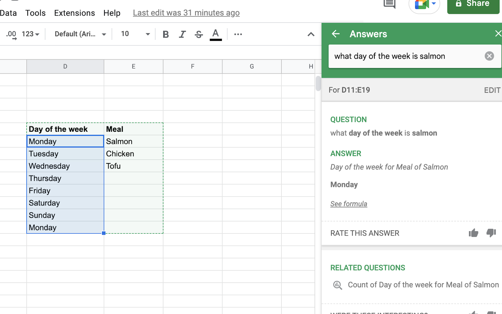
A Google Sheet with a meal plan on it. On the right-hand side, someone asked asked the question "What day of the week is salmon" and received the answer "Monday."

Note: This feature is less of a support bot, more of a math wizard. You can ask it “Total sales in December 2022?” but not “How do use conditional formatting?” (Nor can you demand it give you a hug if your data is giving you too much trouble. That’s what your Google Home is for, apparently.)

Also, make sure you’re using the same language you use in your sheet when you speak to Google bot. For example, if you have a column called “Sales,” call it “Sales” in your question and not “money” or another word.

Uncover your productivity with Google Sheets hacks

There’s no doubt that Google Sheets is a powerful tool. And the 8 hacks listed in this article only scratch the surface of what you can do with it.

At the very least, we hope they’ll help you make the most of the platform, while also helping you save time on your next data analysis or research project — so you can spend more time vacationing in potato-shaped Airbnbs.

Interested in more productivity hacks? Check out our tips for Slack, plus ways to eliminate repetitive work that eats up your day.